POLS 1140
Ideology and Issues
Updated Apr 13, 2026
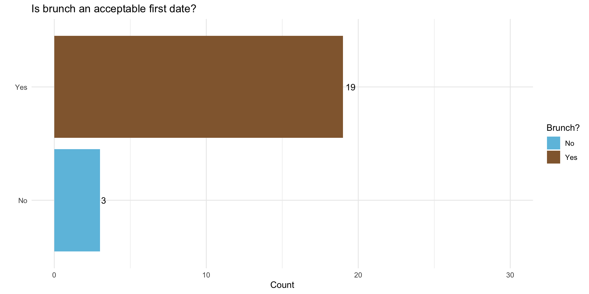
Let’s do brunch?
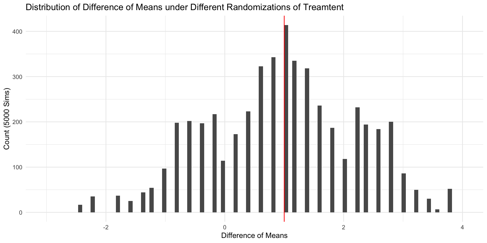
Distribution of Sample ATEs
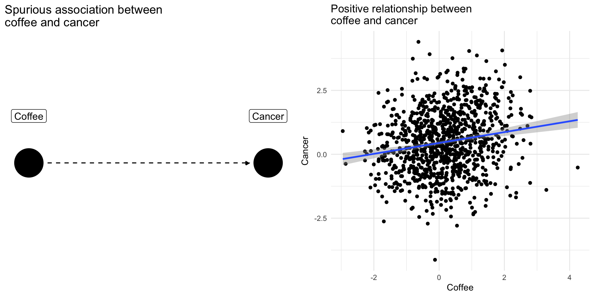
Confounding Bias: The Coffee Example
Drinking coffee doesn’t cause lung cancer we might find correlation between them because they share a common cause: smoking.
Smoking is a confounding variable, that if omitted will bias our results producing a spurious relationsip
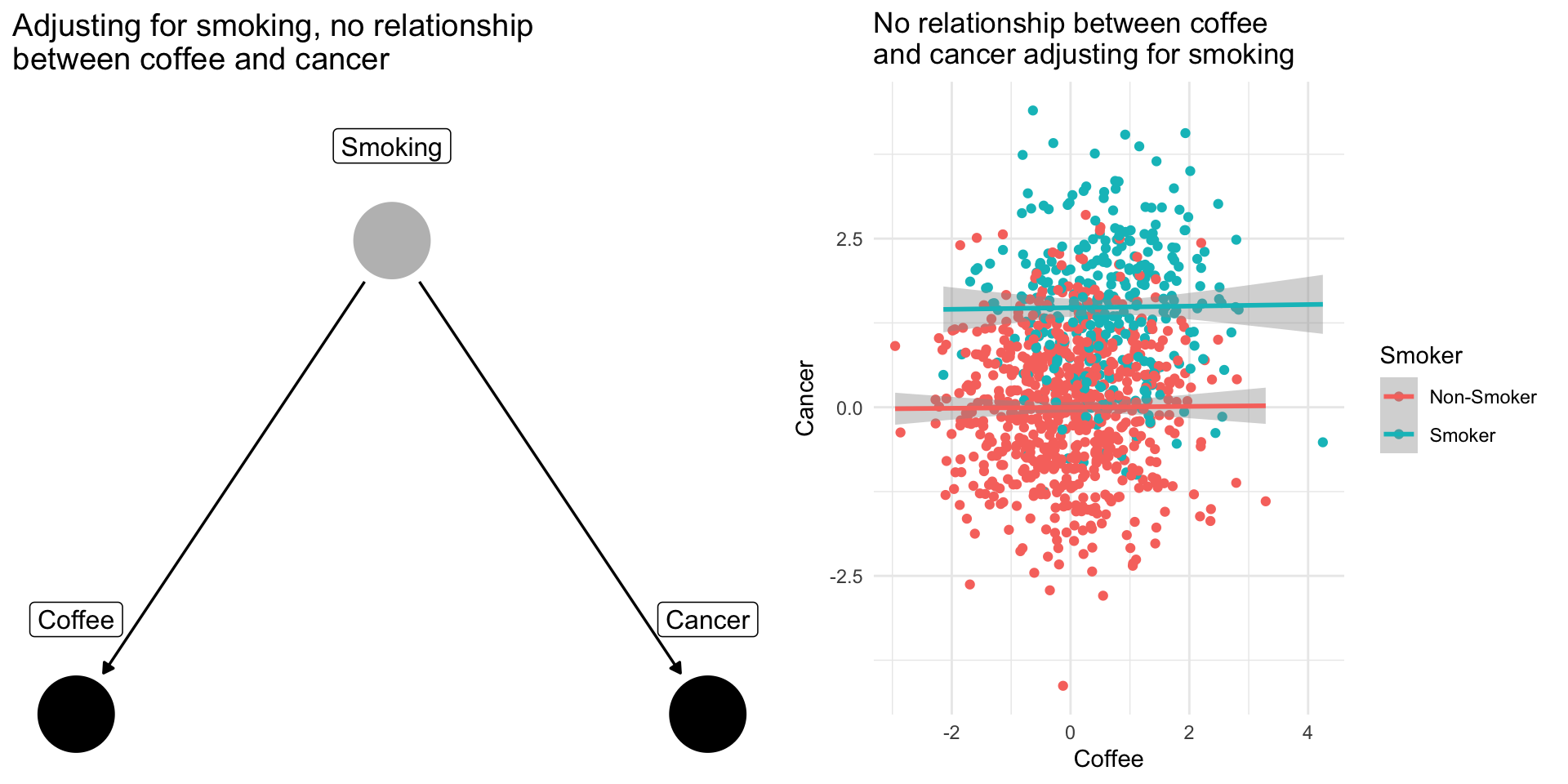
Adjusting for confounders removes this source of bias
Note
When scholars include “control variables” in a regression, often they are trying to adjust for confounding variables that if omitted would bias their results
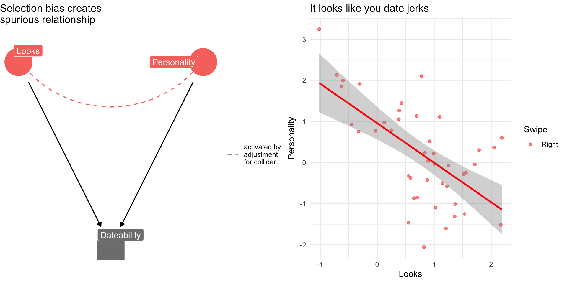
Collider Bias: The Dating Example
Why are attractive people such jerks?
Suppose dating is a function of looks and personality
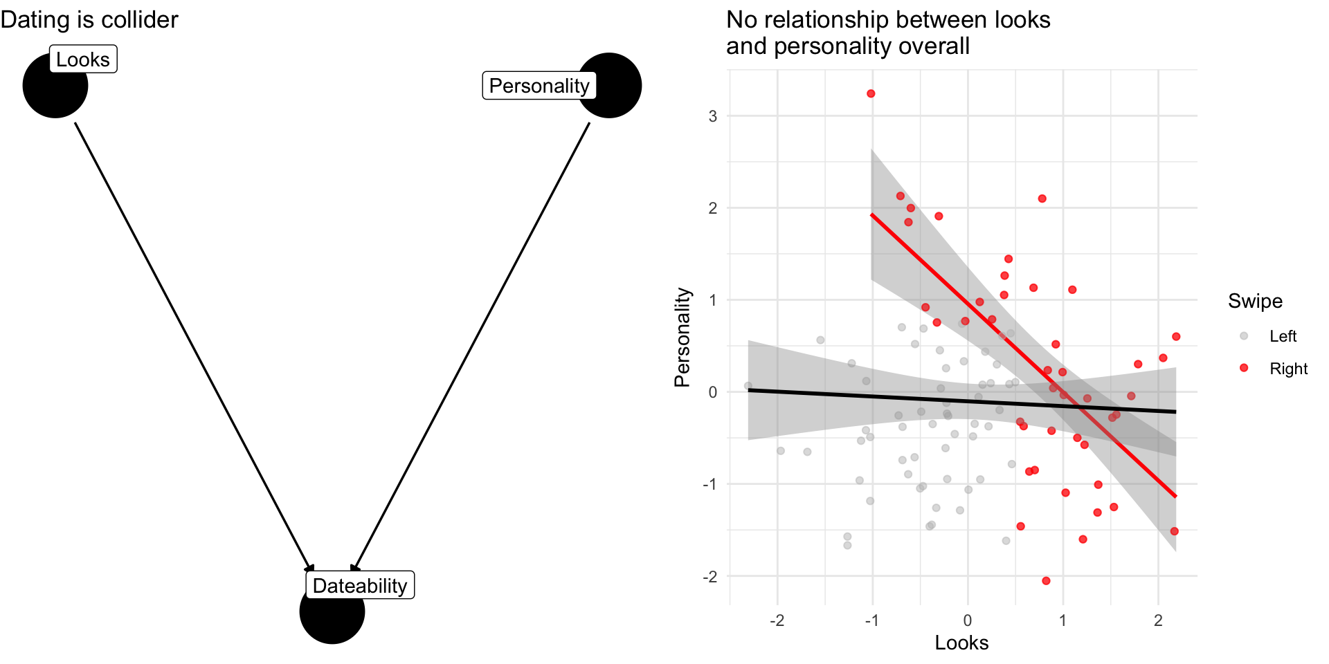
Dating is a common consequences of looks and personality
Basing our claim off of who we date is an example of selection bias created by controlling for collider
Note
If you see a regression model that controls for everything and the kitchen sink without theoretical justification, we might worry about the potential for collider bias
When to control for a variable:

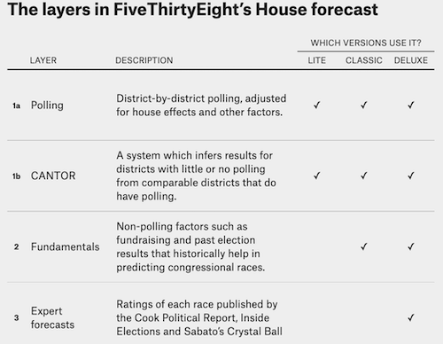
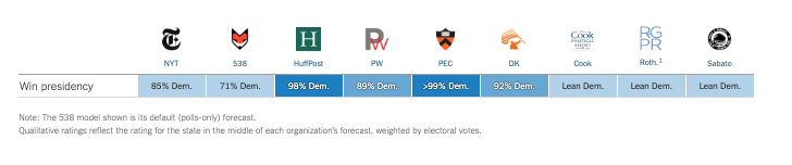
FiveThirtyEight’s Approach to Forecasting
Under Nate Silver…
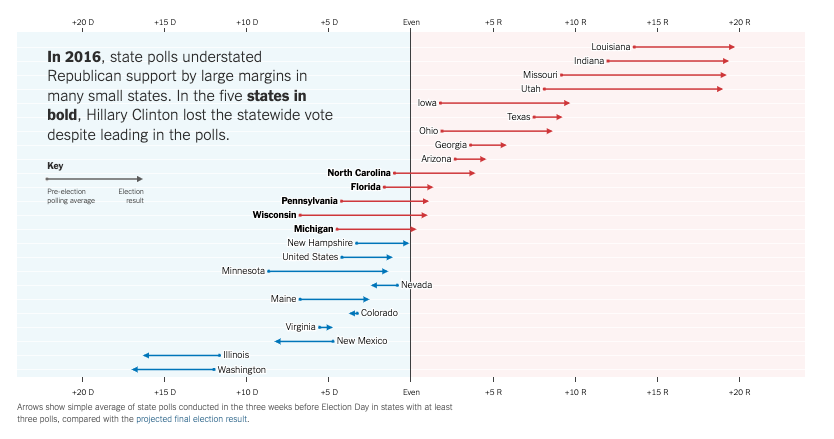
Polling the 2016 Election:
- The polls missed bigly
- National polls were reasonably accurate (Clinton wins Popular Vote)
- State polls overstated Clinton’s lead / understated Trump support
How did we get it so wrong in 2016?
Some likely explanations
Likely voter models overstated Clinton’s support
Large number of undecided voters broke decisively for Trump
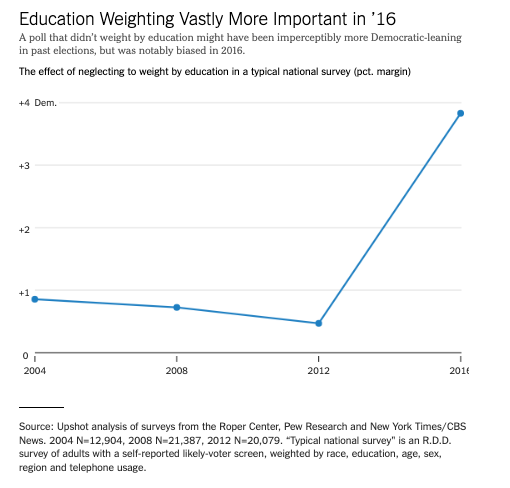
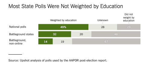
White voters without a college degree underrepresented in pre-election surveys
Weighting for education
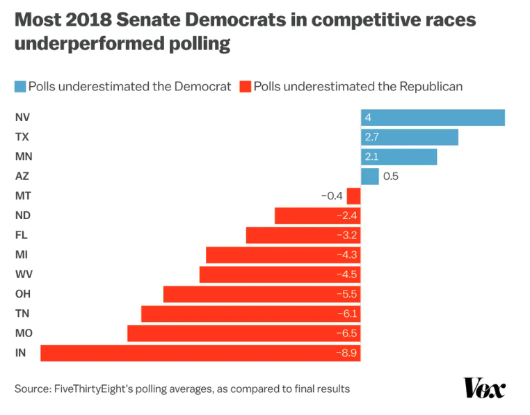
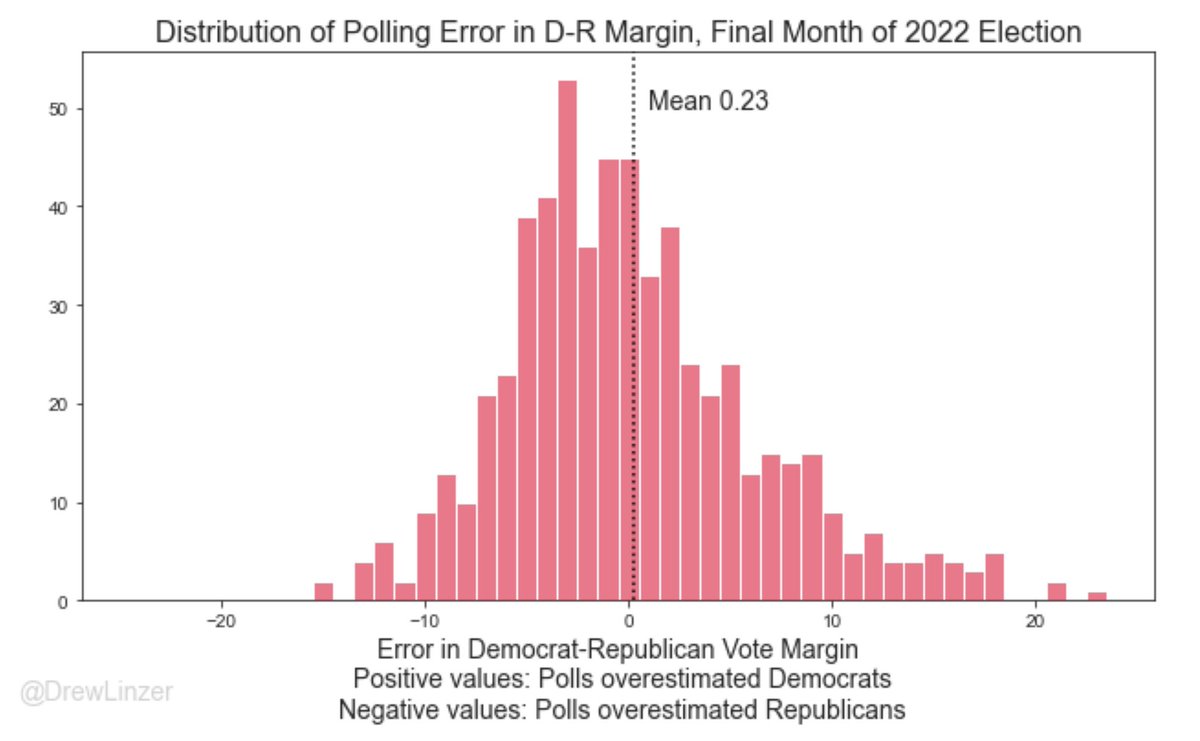
How the polls did in 2022
Overall, pretty good
Average error close to 0
Average absolute error ~ 4.5 percentage points
Some polls tended overstate Republican support (e.g. Trafalgar)
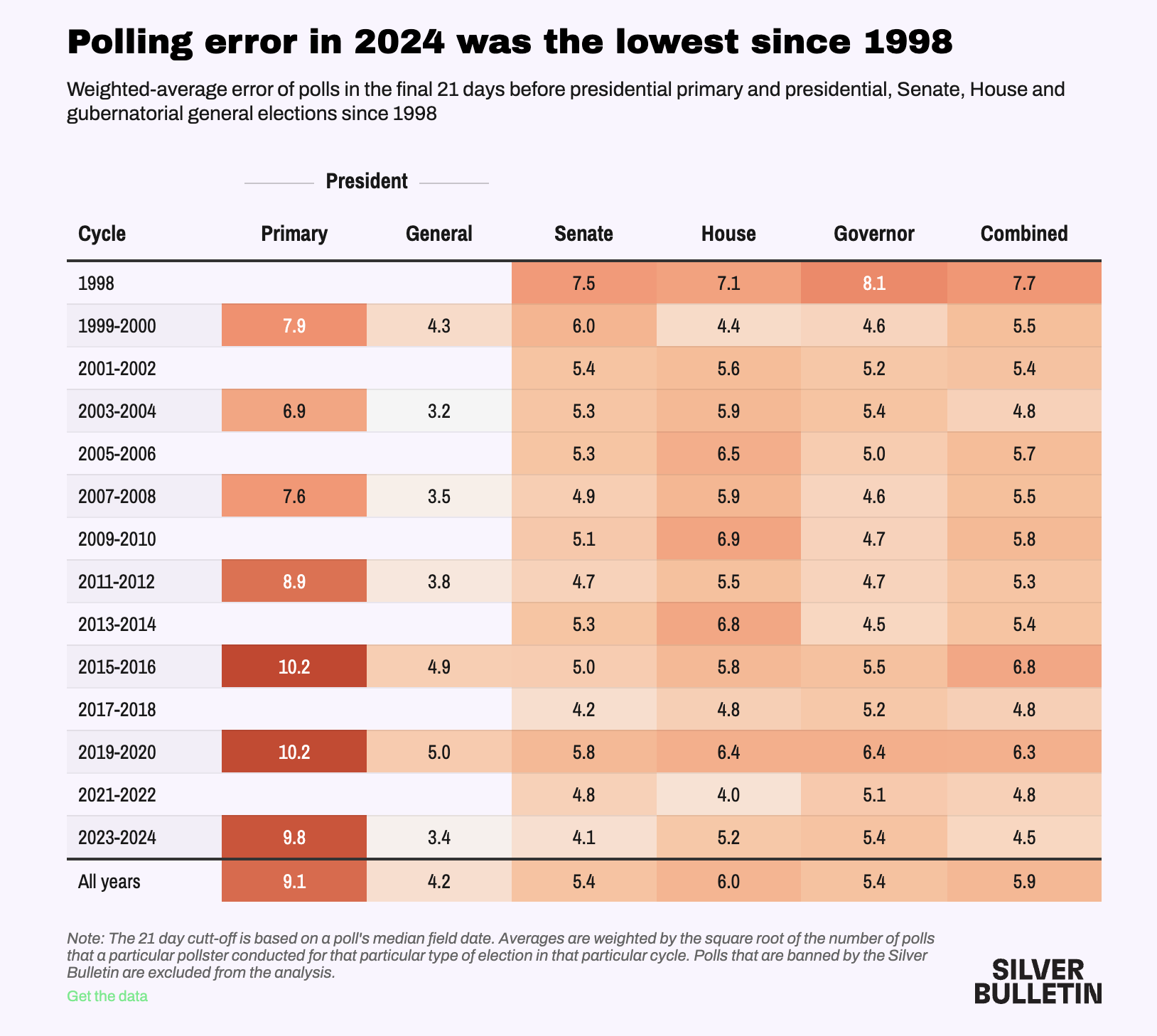
How the polls did in 2024
Good and bad news (Silver Bulletin)
Good:
- Average Polling Error within historical norms
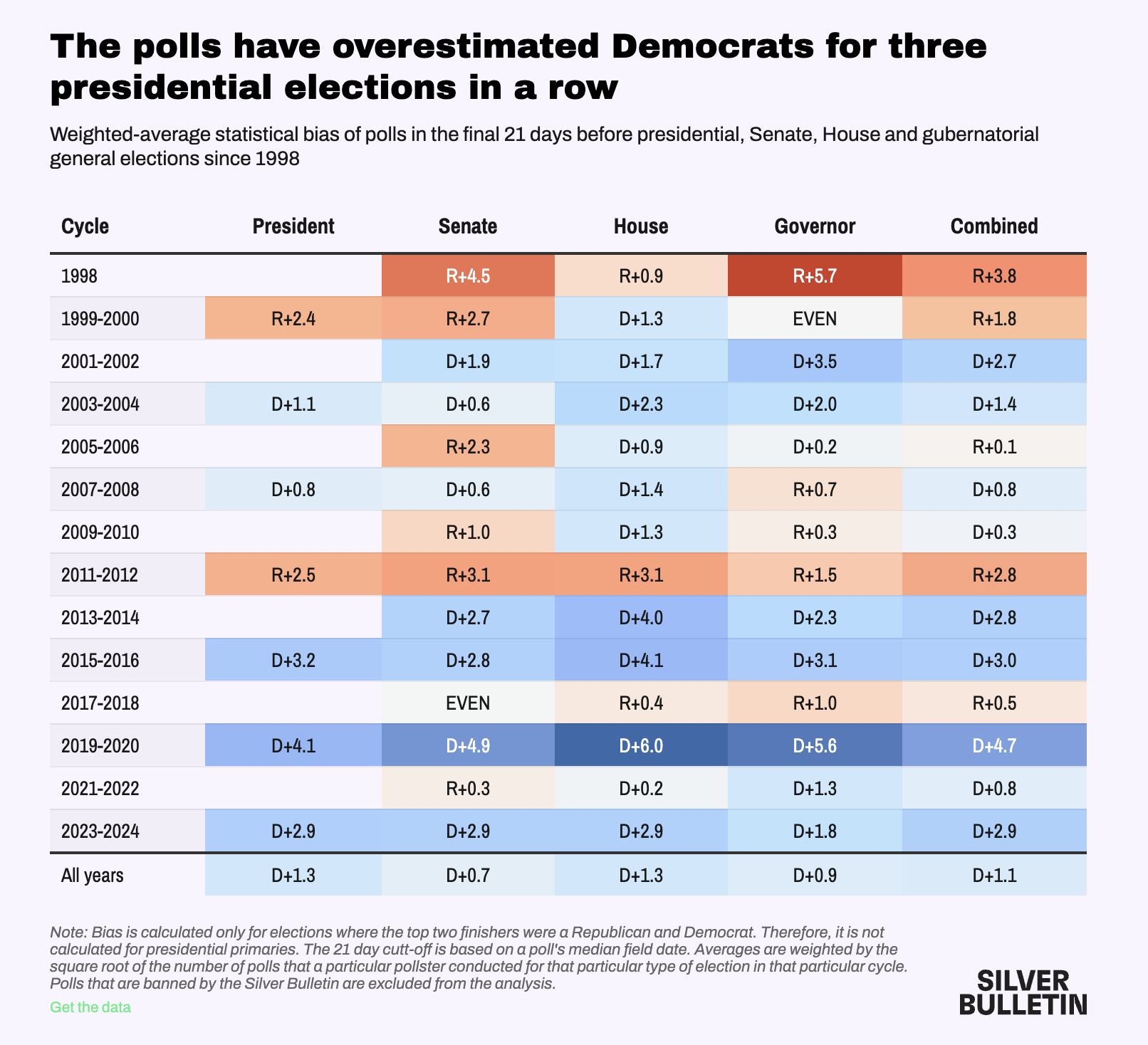
Bad:
Consistently underestimate Trump/Republican support in Presidential election years
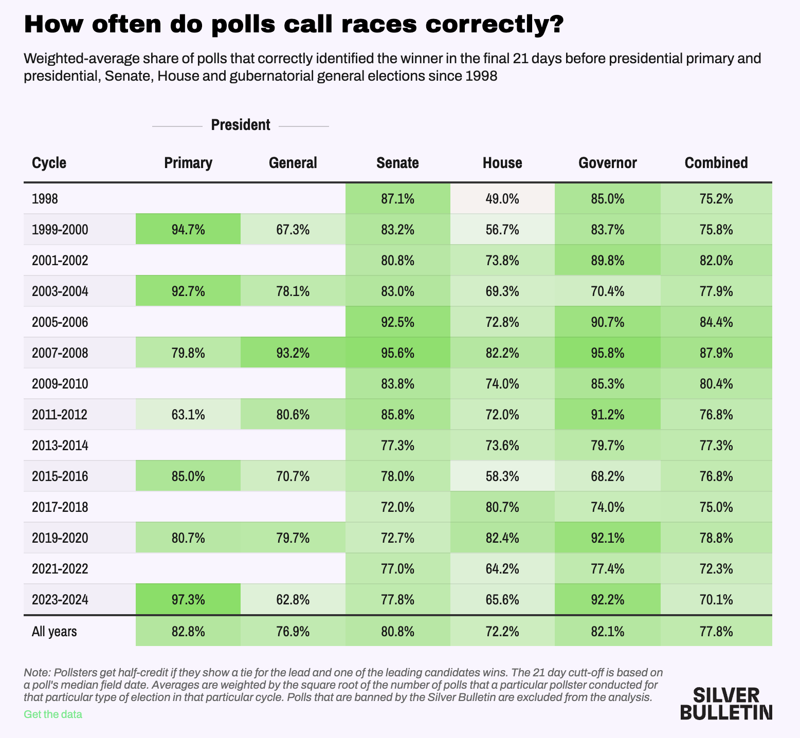
Bad job of calling close races
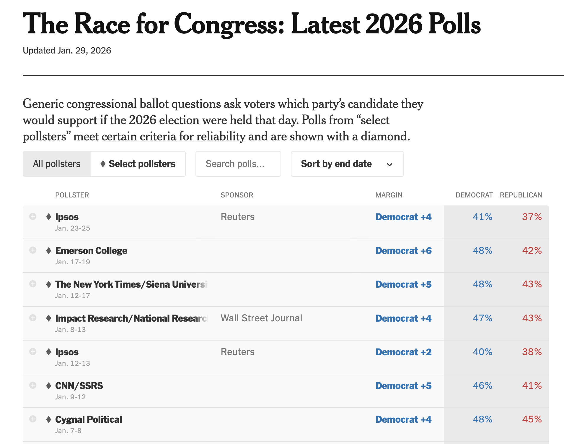
What to expect for 2026 Midterms
Democrats hold a 3-5 point lead in generic ballots
Polling traditionally better when Trumps not on the ballot
Lot’s can change between now and November (Temporal Error…)
Active Use of Ideological Dimensions of Judgement
Recognition of Ideological Dimensions of Judgement
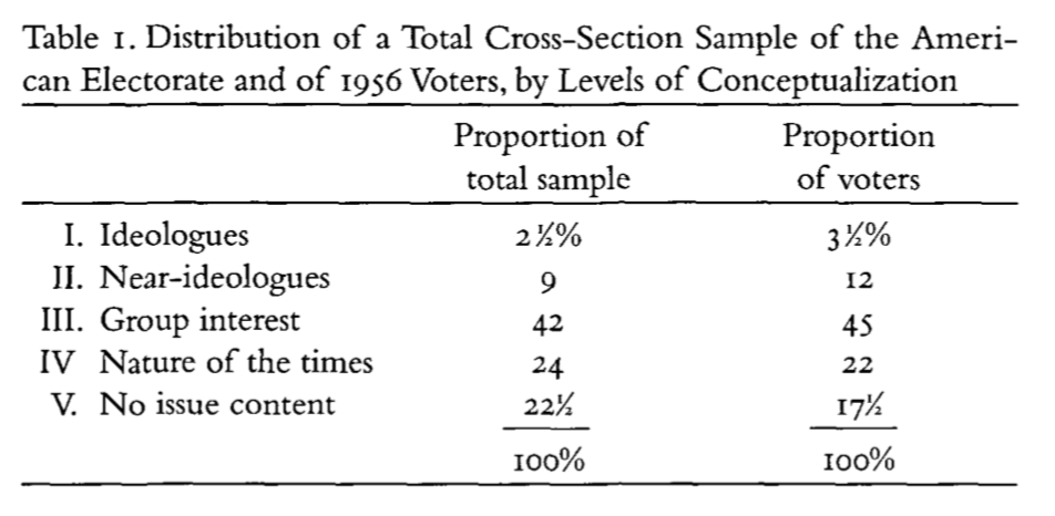
Next Converse considers these levels of conceptualization in 1956 with peoples ability to attach the correct ideological labels with political parties
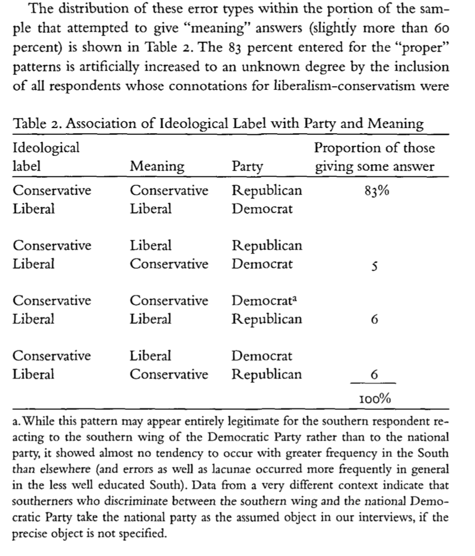
Overall, most respondents label Democrats as the liberal and Republicans as the conservative party (Table 2)
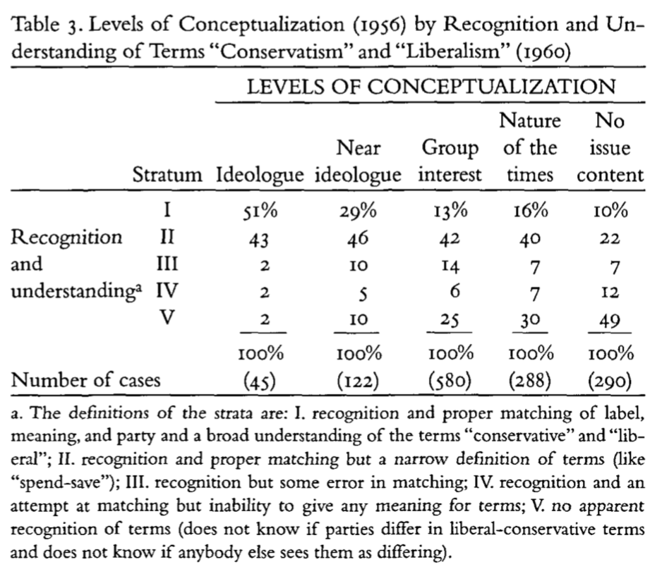
But the depth of this understanding appears quite shallow (e.g. spend vs save) (Table 3)
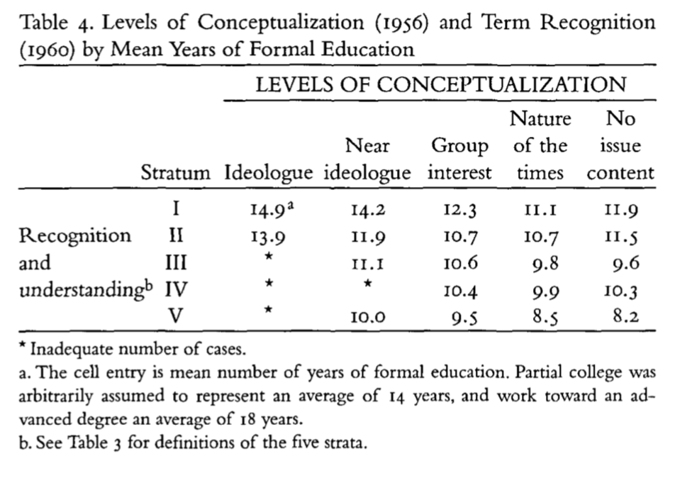
Recognition varies with education (Table 4)
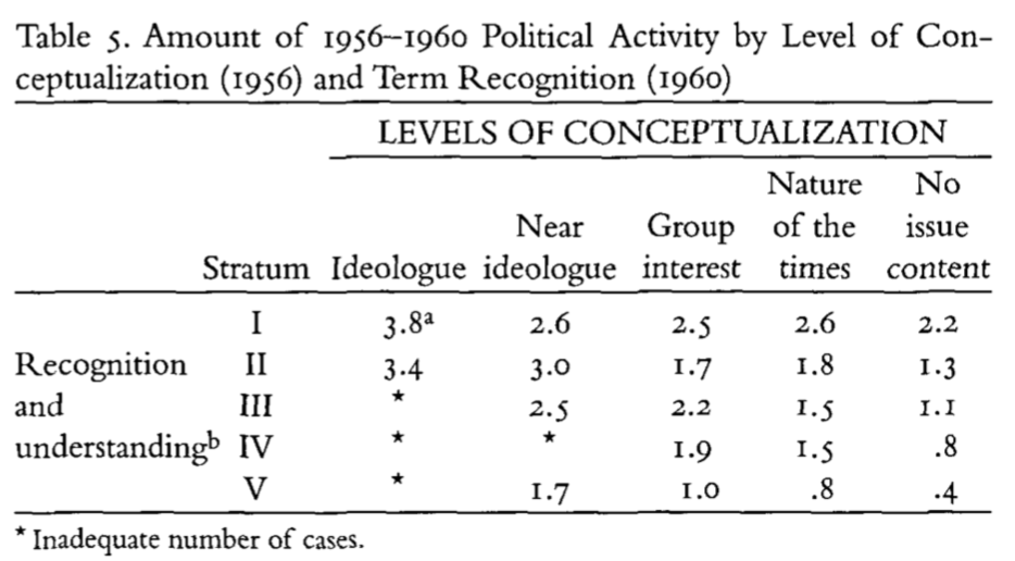
Those with greater levels of recognition are more active in politics (Table 5)
Individuals lack a sense of what goes with what
What are these measures
Read the footnotes!
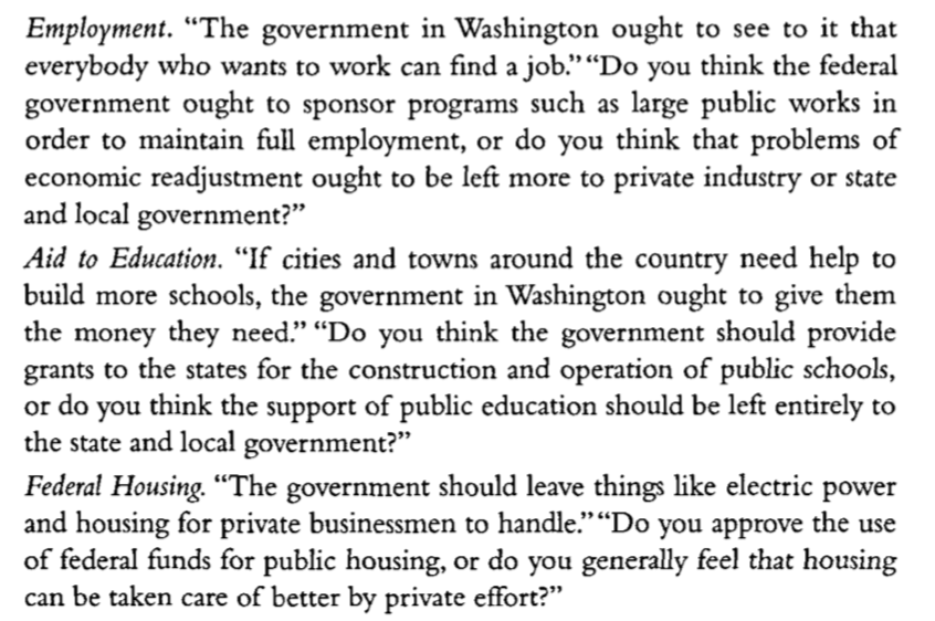
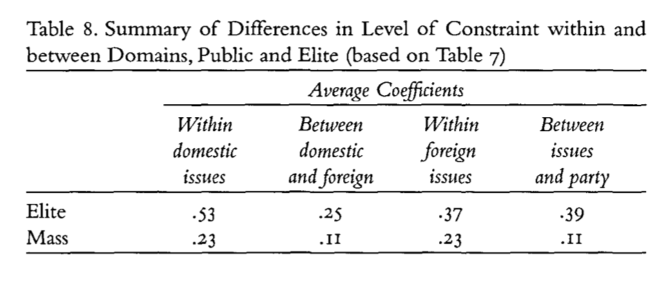
What are these measures
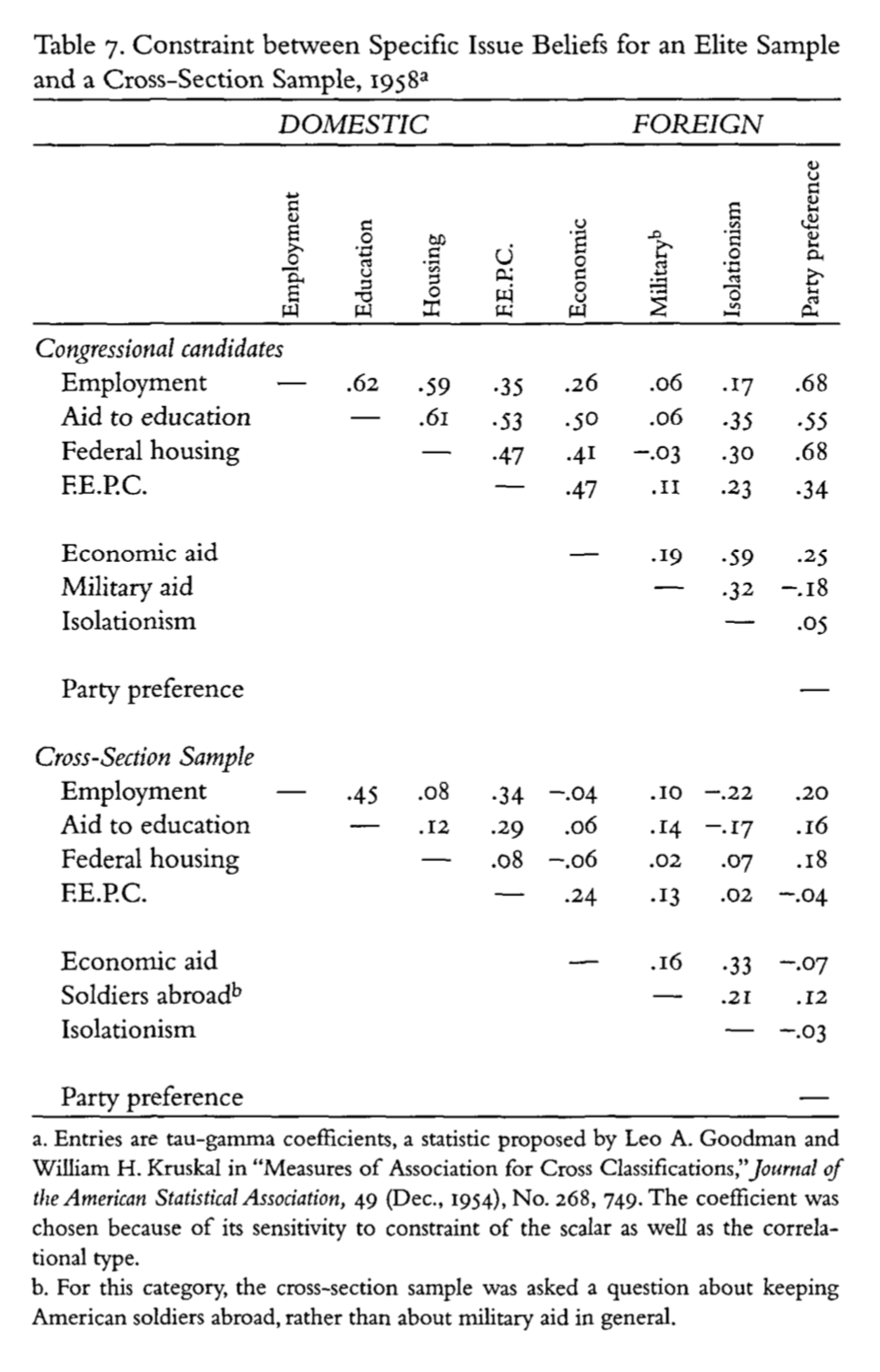
Elites show higher degrees of constraint
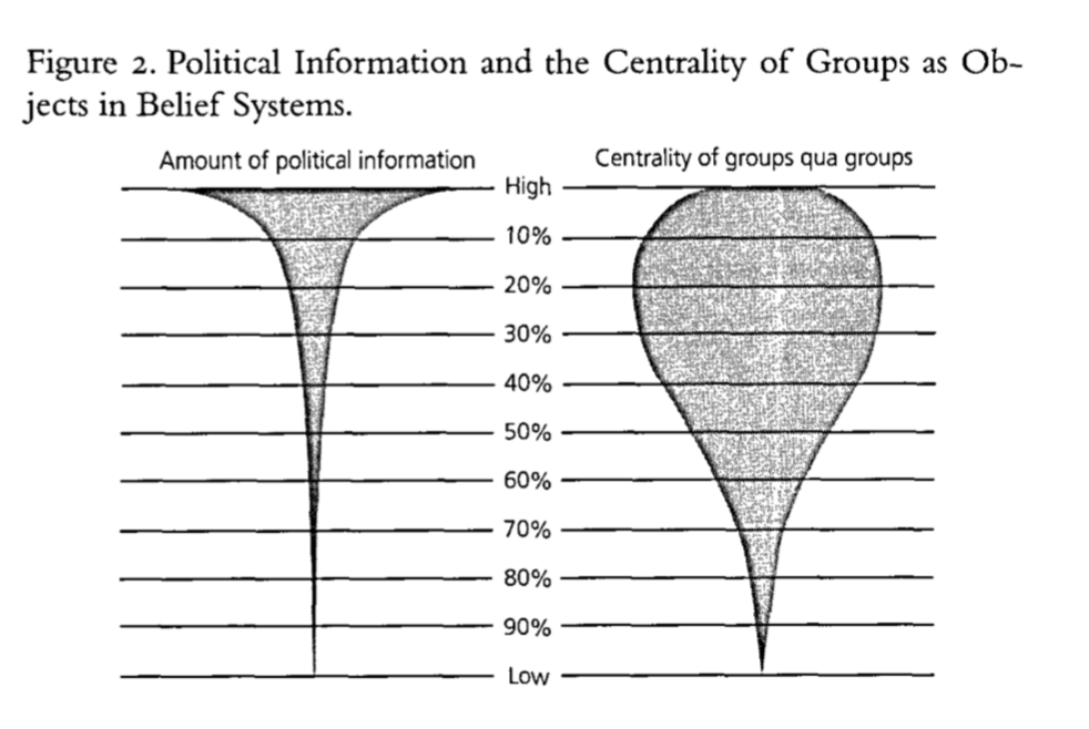
Social groupings as central objects in belief systems
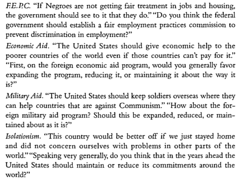
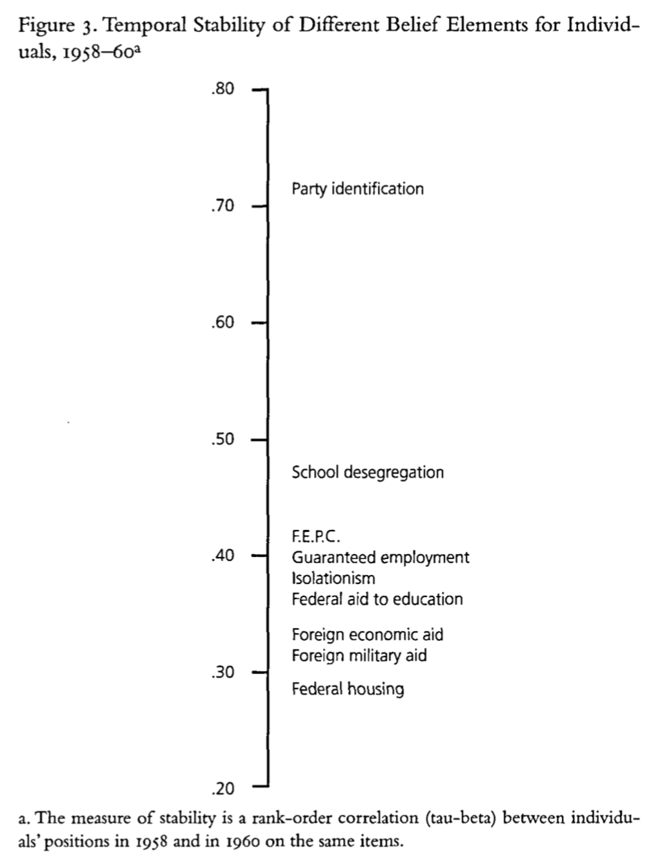
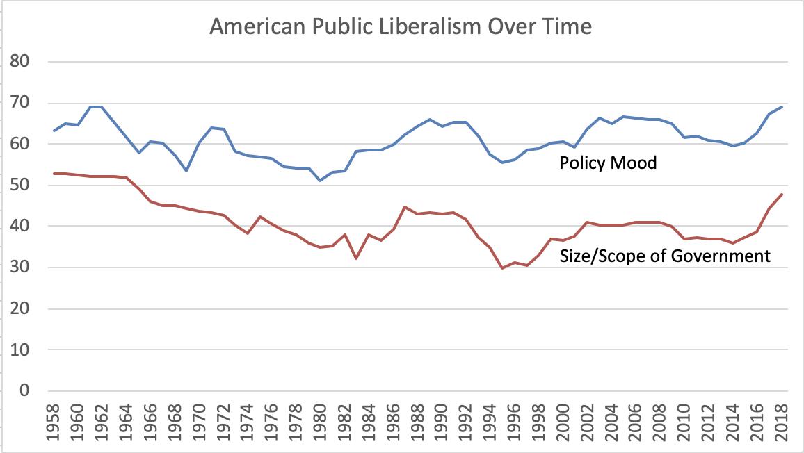
The stability of belief elements over time
Converse considers the stability of responses over time, looking at data from 1958-1960 finding variation the strength of temporal correlations across surveys, and attributes this to the centrality of groups and the party system for the mass public
Responses to Converse (1964)
The Miracle of Aggregation
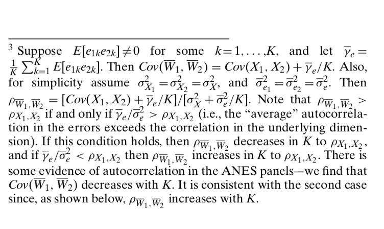
Measurement error reduces reliability
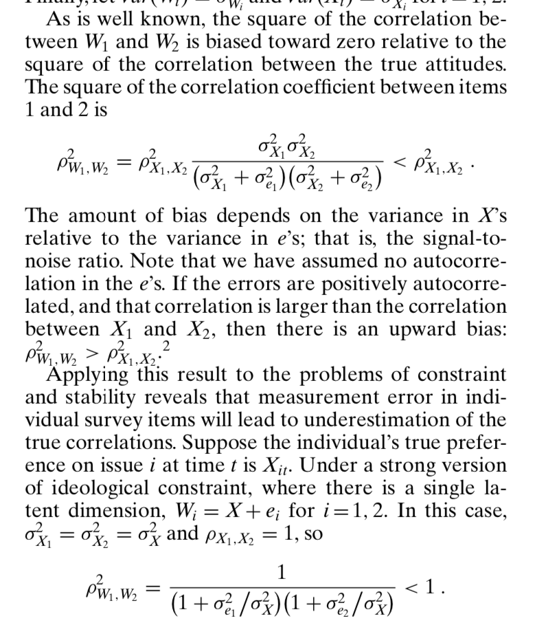
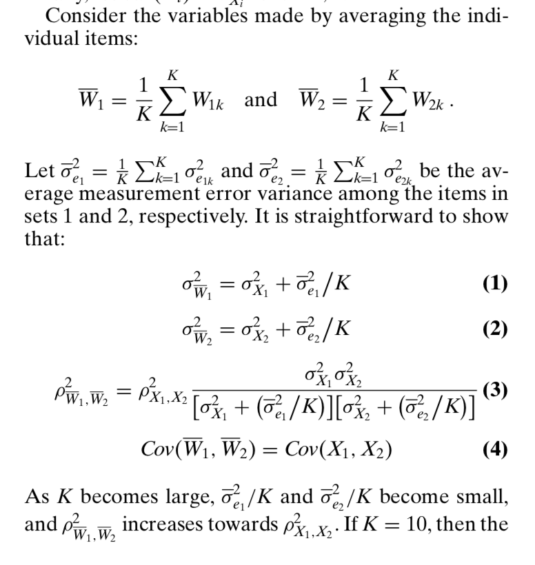
Multiple items reduce measurement error
With some caveats
- No autocorrelation
- Error on one item doesn’t predict error on another
- Additional items can’t be too noisy
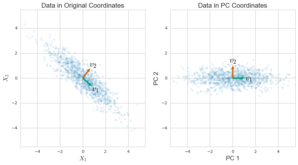
Principal Components Analysis
Find dimensions that explain the maximum variance with the minimum error
A useful tool for data reduction
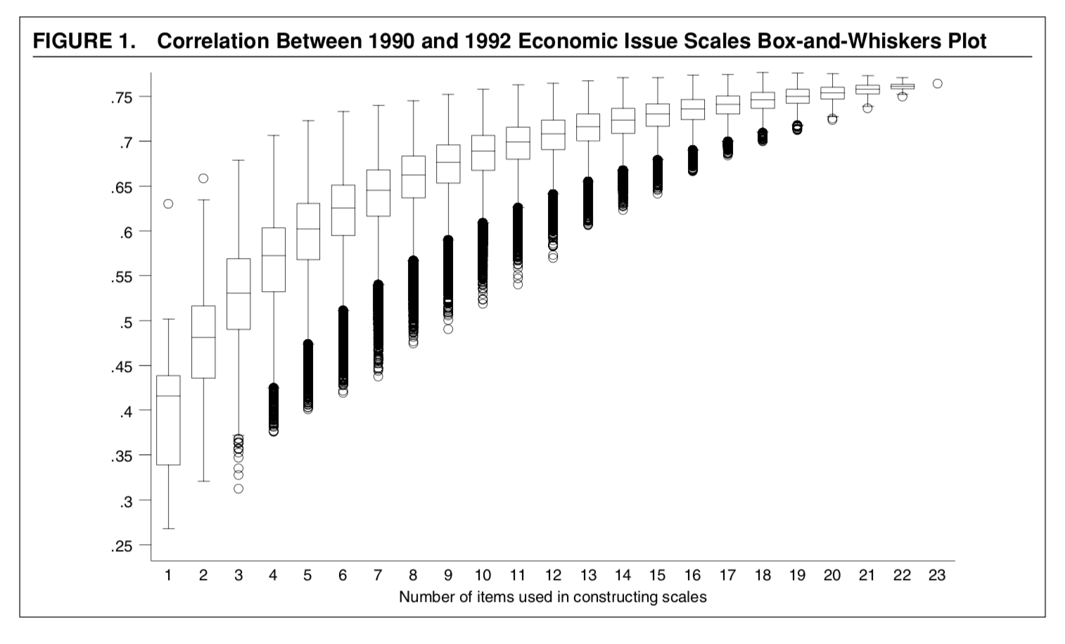
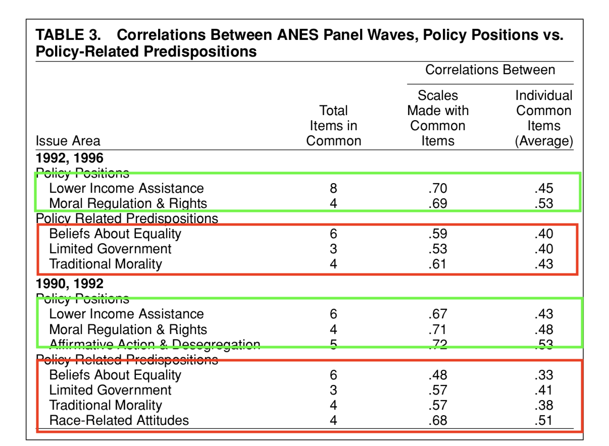
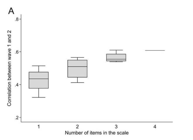
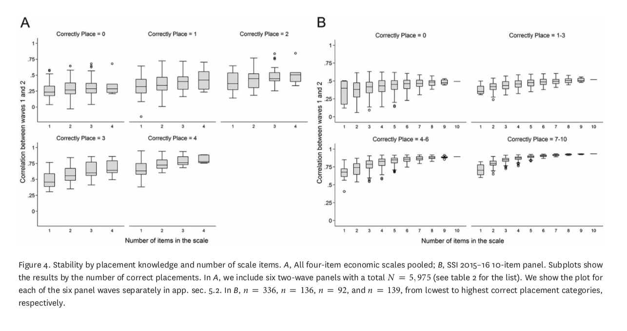
The over time reliability of scales increases with the number of items used
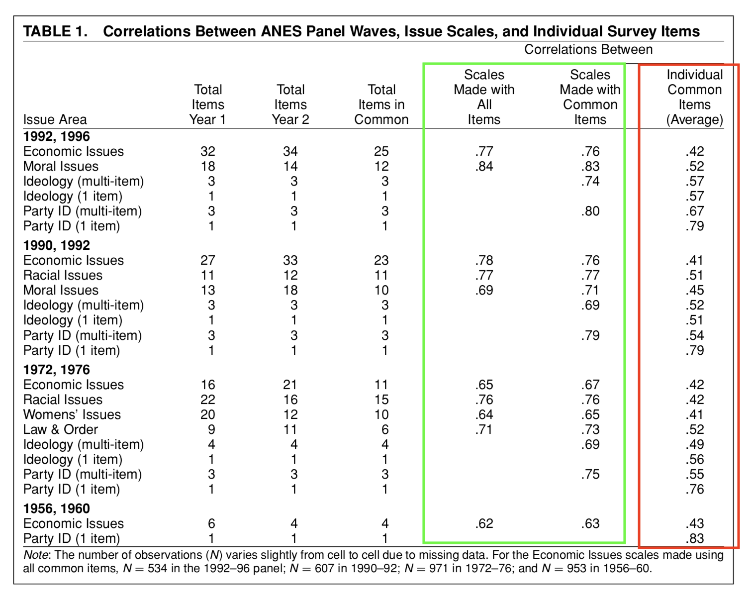
The over time reliability of of scales increases with the number of items used
The correlations are higher between scales within surveys

Issue scales are more stable than policy predispositions
Little variation across political sophistication
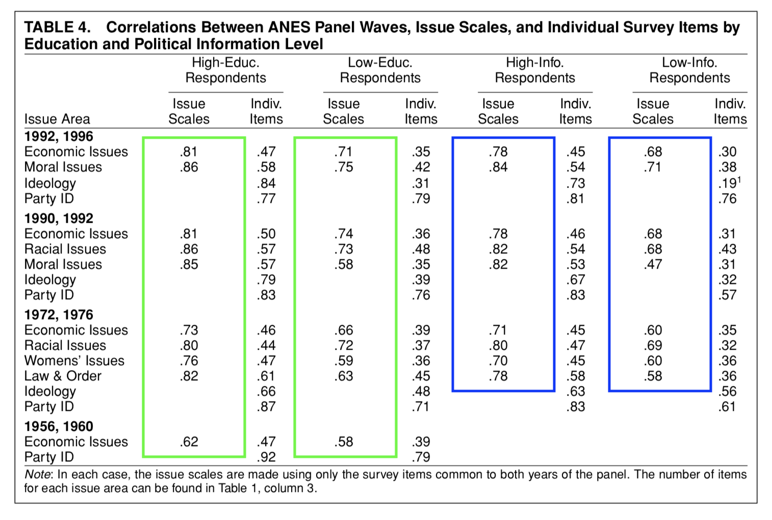
This is in contrast to what Converse’s “Black and White” model would predict and consistent with general arguments about measurement error
The entry point for Freeder et al.’s critique
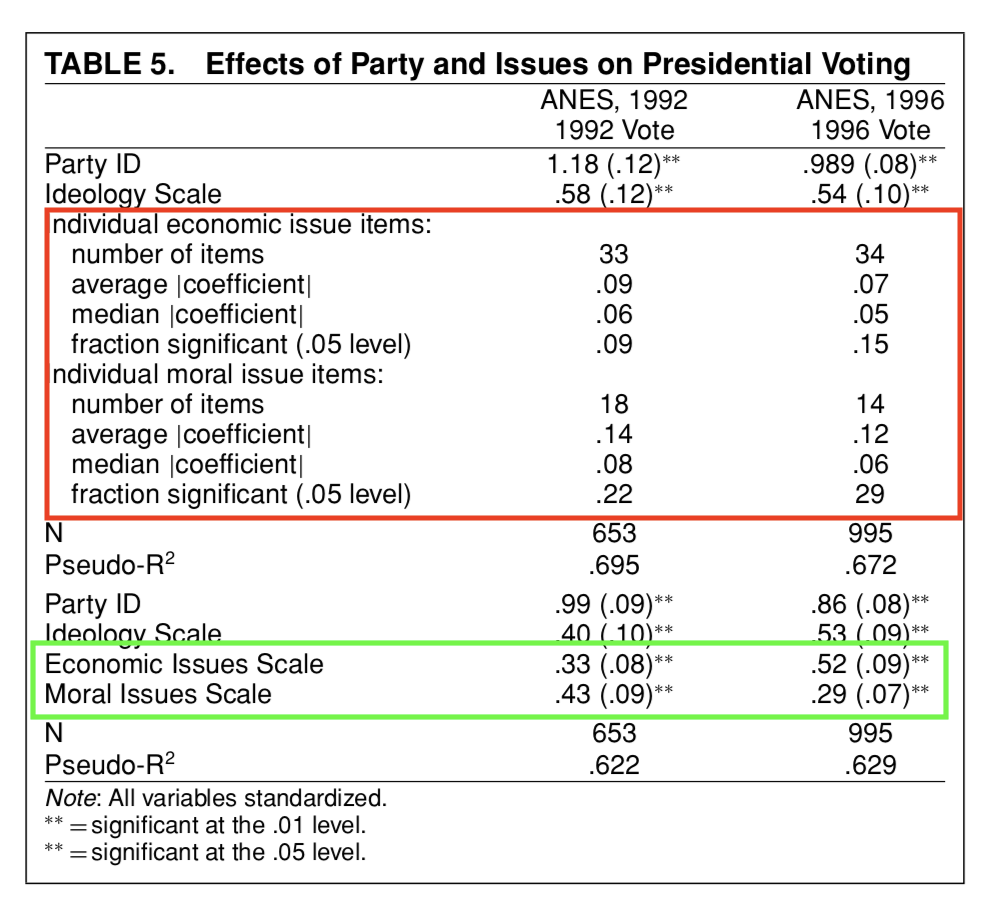
Issue scales predict vote choice
More items reduces measurement error
Constraint doesn’t vary with general knowledge, but does vary with WGWW
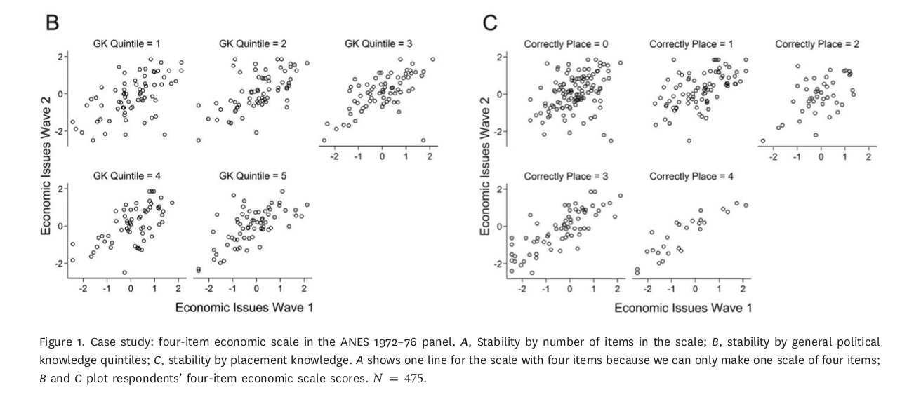
True of scales and individual items
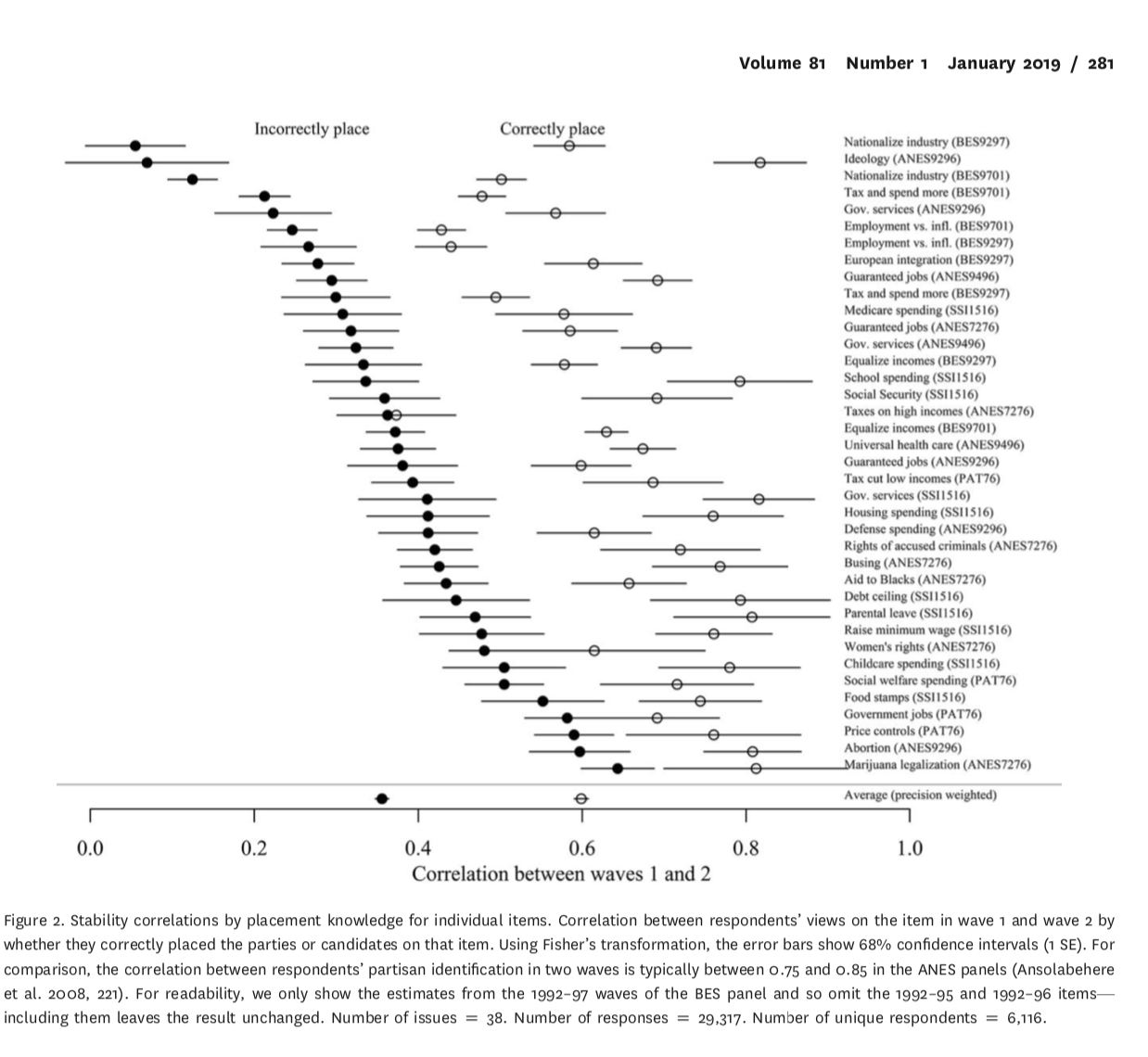
WGWW predicts attitude stability
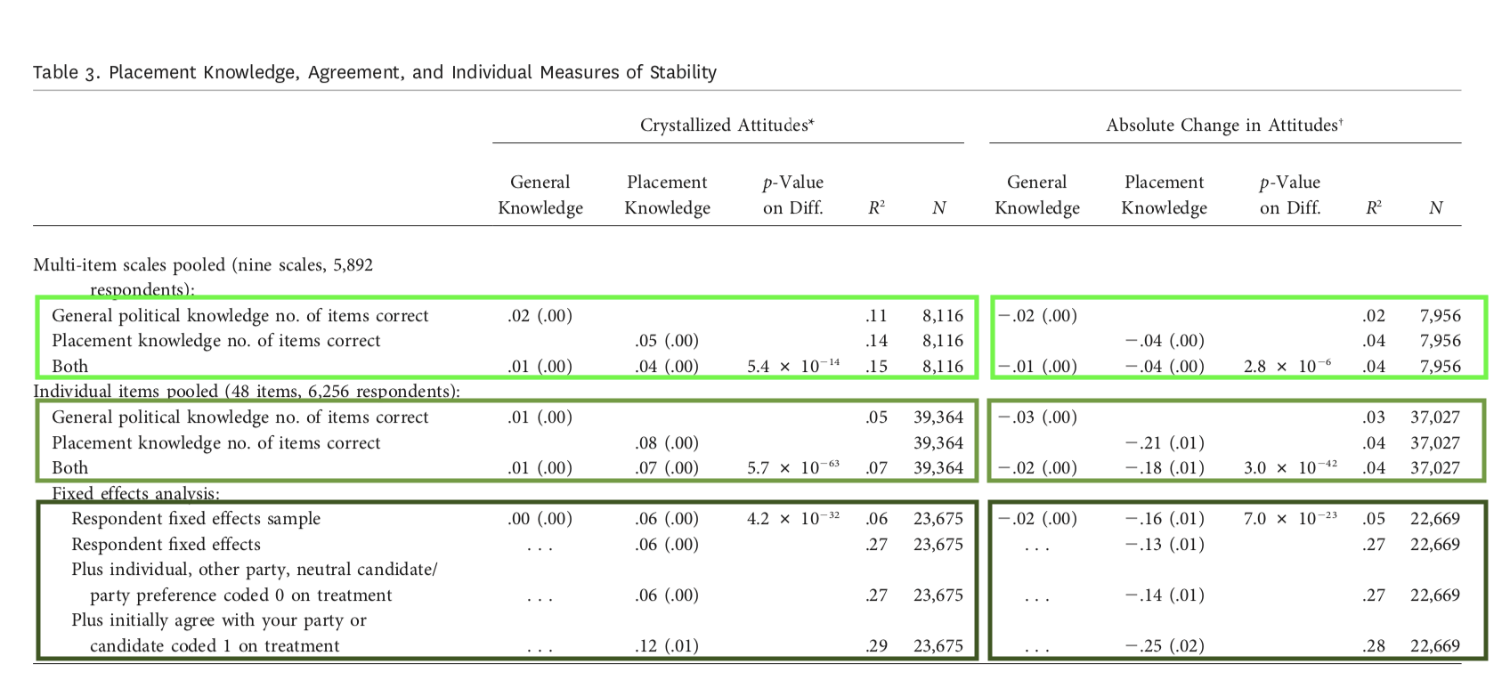
But only for people who agree with their party’s positions

More items won’t fix the problem

Social Groupings as central objects in belief systems